Transmission Shafting Analysis

This page provides the chapter on shaft analysis from the "Stress Analysis Manual," Air Force Flight Dynamics Laboratory, October 1986.

10.1 Introduction to Transmission Shaft Analysis

This section presents design methods for mechanical shafting. In this discussion, a shaft is defined as a rotating member, usually circular, which is used to transmit power. Although normal and shear stresses due to torsion and bending are the usual design case, axial loading may also be present and contribute to both normal and shear stresses. The design case must consider combined stresses.

The general design of shafts will be discussed with emphasis on circular sections, either solid or hollow.

10.2 Nomenclature Used in Transmission Shafting Analysis

C	=	numerical constants
D, d	=	diameter
E	=	modulus of elasticity
fpm	=	feet per minute
F	=	force
G	=	modulus of elasticity in shear
hp	=	horsepower
I	=	moment of inertia
J	=	polar moment of inertia
k	=	radius of gyration
K	=	stress concentration factor, normal stress
K_t	=	stress concentration factor, shear stress
L	=	length
M	=	bending moment

n	=	revolutions per minute
r	=	radius
rpm	=	revolutions per minute
f	=	normal stress
f_e	=	endurance limit stress, reversed bending
f_s	=	shearing stress
f_yp	=	yield point stress, tension
SAE	=	Society of Automotive Engineers
T	=	torque
V	=	velocity, feet per minute
y	=	deflection
α	=	column factor
ϕ	=	(phi) angular deformation
ω	=	(omega) angular velocity, radians per second

10.3 Loadings on Circular Transmission Shafting

Transmission shafting is loaded by belts, chains, and gears which both receive power from prime movers and distribute it to accomplish desired results. Differences in the amount of power either added or subtracted at various points on the shaft result in torsion of the shaft. The driving forces and the driven resistances result in bending of the shaft and, for helical gearing, an axial loading is also produced. These loadings generate both normal and shear stresses in the shaft.

The torsion loading produces a maximum shear stress at the shaft surface calculated from

$$ f_s = {T ~r \over J} $$

(10-1)

where the torque transmitted through the section is determined from the horsepower relation:

$$ T = { hp ~(63,000) \over n } $$

(10-2)

The development of these relations can be found in standard texts.

The bending force produced by gears or chains is equal to the net driving force given by

$$ F = {T \over r} $$

(10-3)

where the radius of the gear or sprocket is used. Bending forces from belts must be obtained from the sum of the forces exerted on each side of the pulley. The usual method is to use the following relation:

$$ F_1 + F_2 = C (F_1 - F_2) $$

(10-4)

where F₁ is the tension side force and F₂ is the slack side force. The quantity (F₁ - F₂) is the net obtained from the horsepower equation. For flat belts, the value of C is between 2 and 3, depending upon conditions of installation. For V-belts, use C = 1.5.

The axial load produced from gearing must be obtained from considerations of the type of gear-tooth design used. It is beyond the scope of this section to elaborate on gear loadings. Suffice it to say that they must be considered.

The bending forces create normal stresses in the shaft given by

$$ f = {M ~r \over I} $$

(10-5)

The axial forces create a normal stress

$$ f = \alpha ~{F \over A} $$

(10-6)

where α is the factor changing F/A into an equivalent column stress where F is compression and there is an appreciable length of unsupported shaft. The recommended values of α are given in the following relation:

$$ \alpha = { 1 \over 1 - 0.0044 ~(L/k) } ~~~ (\text{for} ~L/k \lt 115) $$

(10-7)

$$ \alpha = { f_y ~(L/k)^2 \over C ~\pi^2 E } ~~~ (\text{for} ~L/k \gt 115) $$

(10-8)

C = 1.0 is used for hinged ends and C = 2.25 is used for fixed ends. For tensile axial loads and for short lengths in compression, α = 1.0 is used.

Need Structural Calculators?

We have a number of structural calculators to choose from. Here are just a few:

10.4 Analysis of Combined Stresses in Transmission Shafting

The recommended method for design of ductile materials subjected to combined normal and shear stresses is that employing the maximum shear stress theory. This theory states that inelastic action begins when the shear stress equals the shearing limit of the material. The maximum shear stress at any section is given as follows:

$$ f_{s.max} = \left[ f_s^2 + \left({f \over 2}\right)^2 \right]^{1/2} $$

(10-9)

where f_s and f are obtained from the relations given in Section 10.3. The value to be used for the design maximum shear stress, f_s.max, is discussed in the next section.

10.5 Design Stresses and Load Variations for Transmission Shafting

The design stress is obtained from the yield strength of the material to be used. However, it must be modified to account for various loading anomalies. The ''Code of Design of Transmission Shafting, 11 which has been published by the ASME as code B 1 7c, 192 7, gives the basic factors to be used in determining the design stresses, either normal or shear. According to this code, the basic design stress shall be:

Shear Design Stress	f_s = 0.3 (tensile yield strength), or
	f_s = 0.18 (tensile ultimate strength)

Normal Design Stress	f = 0.6 (tensile yield strength), or
	f = 0.36 (tensile ultimate strength)

The smaller of the two computed stresses is to be used. For combined stresses, as discussed in Section 10.4, the shear design stress is used. The code also applies a factor of 0.75 to the calculated design stress if the section being considered includes a keyway. It is noted that this is equivalent to a stress concentration factor of 1.33. Table 10-2 should also be consulted prior to making allowance for keyways. Although the code does not mention stress concentration factors further, they must be considered in any design.

Figures 10-1 through 10-5 give stress concentration factors to be applied to the design stress for various types of section discontinuities.

Stress Concentration Factor for Solid Shaft with Fillet

Stress Concentration Factor for Solid Shaft with Radial Hole

Stress Concentration Factor for Solid Shaft with Groove

Stress Concentration Factor for Hollow Shaft with Fillet

Stress Concentration Factor for Hollow Shaft with Radial Hole

Tables 10-2 and 10-3 give stress concentration factors to be applied to keyways and several screw thread types. These are applied only if the section being analyzed includes either threads or a keyway.

Table 10-2: Values of Stress Concentration Factor for Keyways, K
	Annealed		Hardened
Type of Keyway	Bending	Torsion	Bending	Torsion
Profile	1.6	1.3	2.0	1.6
Sled-Runner	1.3	1.3	1.6	1.6

Table 10-3: Values of Stress Concentration Factor for Screw Threads, K
	Annealed		Hardened
Type of Thread	Rolled	Cut	Rolled	Cut
American National (square)	2.2	2.8	3.0	3.8
Whitworth, Unified St'd.	1.4	1.8	2.6	3.3
Dordelet	1.8	2.3	2.6	3.3

The code also recommends the application of a shock and fatigue factor to the computed torsional moment or bending moment. This factor accounts for the severity of the loading during stress reversals caused by the revolution of the shaft. Table 10-4 gives these factors for rotating shafts.

Table 10-4: Values of Shock and Fatigue Factors for Rotating Shafts (from ASME Code)
Nature of Loading	K_m (bending)	K_s (torsion)
Gradually Applied or Steady	1.5	1.0
Suddenly Applied, minor	1.5 to 2.0	1.0 to 1.5
Suddenly Applied, heavy	2.0 to 3.0	1.5 to 3.0

Need Structural Calculators?

We have a number of structural calculators to choose from. Here are just a few:

10.6 Design Procedure for Circular Transmission Shafting

The recommended design procedure for circular shafts is as follows:

Define all loads on the shaft.
Determine the maximum torque and its location.
Determine the maximum bending moment and its location.
Determine the design stress.
Determine the shaft diameter at the critical diameter.
Check for shaft deflections.

A sample problem will illustrate the application of the above principles and the previous relations.

10.6.1 Sample Analysis of Circular Transmission Shafting

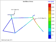
The loaded shaft illustrated in Figure 10-6 receives 20 hp at 300 rpm on pully B at a 45° angle from below. Gear C delivers 8 hp horizontally to the right, and gear E delivers 12 hp downward to the left at 30°. The shafting is to be cold-drawn C1035 with minimum values of tensile yield strength, f_y = 72,000 psi, and of tensile ultimate strength, f_u = 90,000 psi.

The forces shown are those which are placed upon the shaft. The gearing loads do not consider the normal component. This is reasonable for 14-½° tooth design, but for higher pressure angles the side force should be included.

1) Define the loads.

The torques transmitted by the shaft are

$$ T_B = { 63,000 ~hp \over n } = { (63,000) (20) \over 300 } = 4200 ~\text{in-lbs} $$

(10-10)

on shaft between B and C.

$$ T_C = { (63,000) (8) \over 300 } = 1680 ~\text{in-lbs} $$

(10-11)

taken off at C.

$$ T_E = { (63,000) (12) \over 300 } = 2520 ~\text{in-lbs} $$

(10-12)

on shaft between C and E.

The bending forces from the pulley is given by

$$ F_B = 2 (F_1 - F_2) = {2 T_B \over r_B} = {2 (4200) \over 12} = 700 ~\text{lbs} $$

(10-13)

The bending force from gear C is

$$ F_C = {T_C \over r_c} = {1680 \over 9} = 187 ~\text{lbs} $$

(10-14)

and from gear E, it is

$$ F_E = {T_E \over r_E} = {2520 \over 6} = 420 ~\text{lbs} $$

(10-15)

These applied loads are resolved into their vertical and horizontal components and the bearing reactions calculated. These reactions are found by summing moments and forces in the two planes. From these computations, the shear diagram shown in Figure 10-7 were constructed.

Drawing Illustrating Construction of Shear Diagrams

The maximum bending moment is located where the shear diagram crosses the axis. More complex loadings have several crossing points. Each should be investigated to find the maximum. For the present case, the maximum bending moment in the horizontal plane is

$$ M_{B.x} = (12) (484) = 5810 ~\text{in-lbs} $$

(10-16)

and in the vertical plane it is

$$ M_{B.y} = (12) (419) = 5030 ~\text{in-lbs} $$

(10-17)

Since both of these maximums are at the same place, at pulley B, this is the point of maximum moment for the shaft. It is given by

$$ M_B = \left[ M_{B.x}^2 + M_{B.y}^2 \right]^{1/2} $$

(10-18)

$$ M_B = \left[ (5810)^2 + (5030)^2 \right]^{1/2} $$

(10-19)

$$ M_B = 7685 ~\text{in-lbs} $$

(10-20)

It is observed that if the location of the maximum moments is not the same in each plane, both locations must be checked to find the maximum. It is also observed that for this example the maximum torque is also located at the same section.

The design stress is now determined. Based on the tensile yield strength, the shearing stress is

$$ f_s = (0.3) (72,000) = 21,600 ~\text{psi} $$

(10-21)

and based on tensile ultimate strength, it is

$$ f_{s.design} = (0.18) (90,000) = 16,200 ~\text{psi} $$

(10-22)

Our design will be based on the smaller. An allowance for the keyway is now made. According to the code, 75% of the above stress is used. Thus,

$$ f_{s.design} = (0.75) (16,200) = 12,150 ~\text{psi} $$

(10-23)

The shock and vibration factors to be applied to the torque and moments for a gradually applied loading are K_s = 1.0 and K_m = 1.5; these are obtained from Table 10-4.

It is noted that if the section includes any other type of stress raiser such as a step in the shaft, a radial hole, or a groove, the appropriate stress concentration factors are to be applied to the design stress.

As this is a case of combined stress, the principle of maximum shear stress will be used for the design:

$$ f_{s.design} = \left[ f_s^2 + \left({f \over 2}\right)^2 \right]^{1/2} $$

(10-24)

The shear stress f_s is due to the torque of 4200 in-lbs and the normal stress f is due to the bending moment of 7685 in-lbs.

Thus, based on the use of a solid circular shaft,

$$ f_s = { K_s T_c \over J } = { 16 K_s T \over \pi D^3 } = { (16) (1.0) (4200) \over \pi D^3 } $$

(10-25)

$$ f_x = { K_m M_c \over I } = { 32 K_m M \over \pi D^3 } = { (32) (1.5) (7685) \over \pi D^3 } $$

(10-26)

Substituting into Equation (10-24) the above quantities gives

$$ 12,150 = \left\{ \left[{ (16) (1.0) (4200) \over \pi D^3 }\right]^2 + \left[{ (32) (1.5) (7685) \over 2 \pi D^3 }\right]^2 \right\}^{1/2} $$

(10-27)

Solving for D³ gives

$$ D^3 = {16 \over 12.15 \pi} \left\{ (4.2)^2 + [(1.5)(7.685)]^2 \right\}^{1/2} $$

(10-28)

and

$$ D = 1.726 ~\text{in} $$

(10-29)

The closest size commercial shafting is 1-15/16 in. It is noted that commercial power transmission shafting is available in the following sizes:

15/16, 1-3/16, 1-7/16, 1-11/16, 1-15/16, 2-3/16, 2-7/16, 2-15/16, 3-7/16, 3-15/16, 4-7/16, 4-15/16, 5-7/16, 5-15/16, 6-1/2, 7, 7-1/2, 8

The use of standard sizes facilitates the selection of bearings, collars, couplings, and other hardware.

Machinery shafting, those used integrally in a machine, is available in the following sizes:

By 1/16 in. increments in this range	1/2 to 1 in., tolerance of -0.002 in.
	1-1/6 to 2 in., tolerance of -0.003 in.
	2-1/6 to 2-1/2 in., tolerance of -0.004 in.
By 1/8 in. increments	2-5/8 to 4 in., tolerance of -0.004 in.
By 1/4 in. increments	4-1/4 to 6 in., tolerance of -0.005 in.
By 1/4 in. increments	6-1/4 to 8 in., tolerance of -0.006 in.

Returning to our example, the diameter of the shaft determined is based on strength considerations alone. As deflections are also a prime consideration, both angular and transverse deflections should be checked.

The torsional deflection of a shaft is given by

$$ \phi = {T L \over G J} $$

(10-30)

where L is the length of shaft between the point of application of the torque and the section being considered.

Although the example given was statically determinate, many situations encountered in practice are indeterminate. For these, the location of the maximum stress must be determined by methods of analysis for continuous beams: the area-moment method, the three-moment method, the method of superposition, and the moment-distribution method. The exposition of these methods is covered in the section of this manual devoted to beam analysis.

10.6.2 General Design Equation for Circular Transmission Shafting

A general design equation for circular shafts, both solid and hollow, can be developed on the basis of the recommended procedures. It is

$$ D^3 = { 16 \over f_s \pi (1 - B^4) } \left\{ K_s^2 T^2 + \left[ K_m M + {\alpha F D (1 + B^2) \over 8 } \right]^2 \right\}^{1/2} $$

(10-31)

where B = D_i/D and D_i is the inside diameter of the hollow shaft. This equation requires several trials for solution because of the inclusion of the axial load F.

It is also pointed out that in the design of large-size shafting, the weight of all pulleys and gears should be included in the design calculations.